Ever since the launch of OpenAI’s ChatGPT, everyone is getting mad at learning AI and ML. Not just stopping there, they want to build and release a AI product on their own to mark their position in the global competition. Even those who own a SaaS product earlier, wants to integrate AI & ML features in their product to retain their customers and to be competitive in the global market. In this blog, we’ll learn about building a Linear Regression Model, which is considered to be the very basics of Machine Learning, to place our first step into this competitive market.
Table of Contents
Linear Regression
Linear Regression is a Supervised Learning method, where the predicted output will be continuous in nature. Eg. Price prediction, marks prediction, etc.
Linear Regression is a fundamental statistical and machine learning technique used for modeling the relationship between a dependent variable (also known as the target or response variable) and one or more independent variables (predictors or features). It aims to establish a linear equation that best represents the association between these variables, allowing us to make predictions and draw insights from data.
The primary goal of linear regression is to find the “best-fit” line (or hyperplane in higher dimensions) that minimizes the difference between the predicted values and the actual observed values. This best-fit line is defined by a linear equation of the form:
Y=b0+b1X1+b2X2+…+bnXn
In this equation:
- Y represents the dependent variable we want to predict.
- X1,X2,…,Xn are the independent variables or features.
- b0 is the intercept (the value of Y when all X values are zero).
- b1,b2,…,bn are the coefficients that determine the relationship between each independent variable and the dependent variable.
Linear regression assumes that there is a linear relationship between the predictors and the target variable.
The goal of the model is to estimate the coefficients (b0,b1,…,bn) that minimize the sum of the squared differences between the predicted values and the actual values in the training data. This process is often referred to as “fitting the model.”
Evaluation Metrics
The evaluation metrics of Linear Regression model are as follows,
- Coefficient of Determination or R-Squared (R2)
- Root Mean Squared Error (RSME)
R-Squared
R-Squared describes the amount of variation that is captured by the developed model. It always ranges between 0 & 1. Higher the value of R-squared, the better the model fits with the data.
Root Mean Squared Error
RMSE measures the average magnitude of the errors or residuals between the predicted values generated by a model and the actual observed values in a dataset. It always ranges between 0 & positive infinity. Lower RMSE values indicate better predictive performance.
Car Price Prediction – Example
In this example, we’ll try to predict the car price by building a Linear Regression model. I found this problem and the dataset in Kaggle. I noticed that there’s a submission for this problem, which was perfect. In fact I built my solution by taking a part of that solution.
Let’s dive into the problem.
We’re given a dataset of used cars, which contains the name of the car, year, selling price, present price, number of kilometers it has driven, type of fuel, type of the seller, transmission, and if the seller is the owner. Our goal is to predict the selling price of the car.
Let’s explore the solution.
Import the required packages
import numpy as np
import pandas as pd
import matplotlib.pyplot as plt
import seaborn as sns
from sklearn.model_selection import train_test_split
from sklearn.preprocessing import StandardScaler
from sklearn.linear_model import LinearRegression
from sklearn import metrics
from sklearn.model_selection import KFold
from sklearn.pipeline import make_pipeline
from statsmodels.stats.diagnostic import normal_ad
from statsmodels.stats.outliers_influence import variance_inflation_factor
from statsmodels.stats.stattools import durbin_watson
from scipy import stats
Import the dataset
You can download the dataset (car data.csv) from Kaggle or you can download it from my Github repo.
df = pd.read_csv('./car data.csv')Pre-process the dataset
The below code shows the columns and their datatype and the number of rows. Our dataset has 9 columns and 301 rows.
df.info()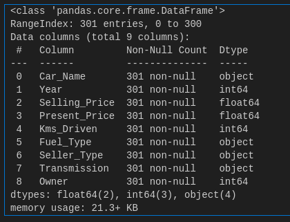
The “Car_Name” column describes the car name. This field should be ignored from our dataset. Because, only the features of the car matters and not it’s name.
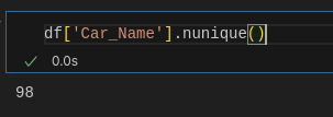
The below code returns the number of unique car names in our dataset.
df['Car_Name'].nunique()We have 98 unique car names in our dataset.
Clearly, it does not add any meaning to our dataset, due to so many categories. Let’s drop that column.
df.drop('Car_Name', axis=1, inplace=True)The dataset has the column named “Year”. Ideally, we need the age of car over the year it was bought / sold. So, let’s convert that to “Age” and remove the “Year” column.
df.insert(0, "Age", df["Year"].max()+1-df["Year"] )
df.drop('Year', axis=1, inplace=True)
“Age” is calculated by finding the difference between the maximum year available in our dataset and the year of that particular car. This is because, our calculations will be specific to that particular time period and to this dataset.
Outliers
An outlier is a data point that differs significantly from other observations. They can cause the performance of the model to drop.
Let’s try to find the outliers in our dataset.
sns.set_style('darkgrid')
colors = ['#0055ff', '#ff7000', '#23bf00']
CustomPalette = sns.set_palette(sns.color_palette(colors))

OrderedCols = np.concatenate([df.select_dtypes(exclude='object').columns.values,
                              df.select_dtypes(include='object').columns.values])

fig, ax = plt.subplots(2, 4, figsize=(15,7),dpi=100)

for i,col in enumerate(OrderedCols):
    x = i//4
    y = i%4
    if i<5:
        sns.boxplot(data=df, y=col, ax=ax[x,y])
        ax[x,y].yaxis.label.set_size(15)
    else:
        sns.boxplot(data=df, x=col, y='Selling_Price', ax=ax[x,y])
        ax[x,y].xaxis.label.set_size(15)
        ax[x,y].yaxis.label.set_size(15)

plt.tight_layout()
plt.show()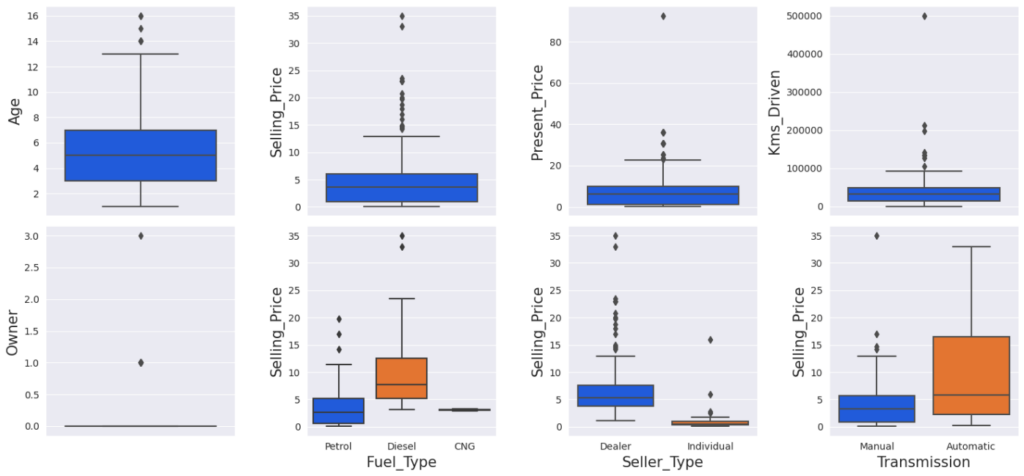
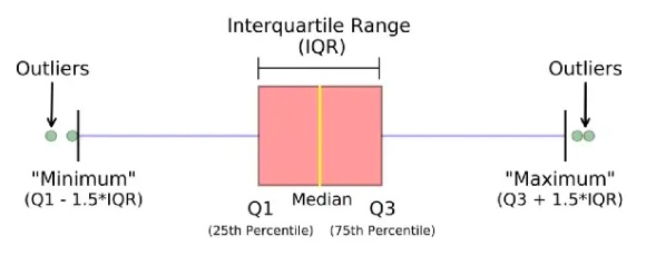
Let’s try to find the outliers using the InterQuartile Range rule.
It is based on the concept of quartiles, which divide a dataset into four equal parts. The IQR (InterQuartile Range rule) rule specifically focuses on the range of values within the middle 50% of the data and uses this range to identify potential outliers.
outliers_indexes = []
target = 'Selling_Price'

for col in df.select_dtypes(include='object').columns:
    for cat in df[col].unique():
        df1 = df[df[col] == cat]
        q1 = df1[target].quantile(0.25)
        q3 = df1[target].quantile(0.75)
        iqr = q3-q1
        maximum = q3 + (1.5 * iqr)
        minimum = q1 - (1.5 * iqr)
        outlier_samples = df1[(df1[target] < minimum) | (df1[target] > maximum)]
        outliers_indexes.extend(outlier_samples.index.tolist())


for col in df.select_dtypes(exclude='object').columns:
    q1 = df[col].quantile(0.25)
    q3 = df[col].quantile(0.75)
    iqr = q3-q1
    maximum = q3 + (1.5 * iqr)
    minimum = q1 - (1.5 * iqr)
    outlier_samples = df[(df[col] < minimum) | (df[col] > maximum)]
    outliers_indexes.extend(outlier_samples.index.tolist())

outliers_indexes = list(set(outliers_indexes))
print('{} outliers were identified, whose indices are:\n\n{}'.format(len(outliers_indexes), outliers_indexes))
By running the above code, we found that there are 38 outliers in our dataset.

However, it’s not always a right decision to remove the outliers. They can be legitimate observations and it’s important to investigate the nature of the outlier before deciding whether to drop it or not.
We are allowed to delete outliers in two cases:
- Outlier is due to incorrectly entered or measured data
- Outlier creates a significant association
Let’s dig even more and find the perfect outliers.
To do that, let’s assume that if the selling price more than 33 Lakhs or if the car has been driven more than 400000 Kilometers are outliers and mark them in Green color. Save all the indices in the removing_indices variable.
# Outliers Labeling
df1 = df.copy()
df1['label'] = 'Normal'
df1.loc[outliers_indexes,'label'] = 'Outlier'

# Removing Outliers
removing_indexes = []
removing_indexes.extend(df1[df1[target]>33].index)
removing_indexes.extend(df1[df1['Kms_Driven']>400000].index)
df1.loc[removing_indexes,'label'] = 'Removing'

# Plot
target = 'Selling_Price'
features = df.columns.drop(target)
colors = ['#0055ff','#ff7000','#23bf00']
CustomPalette = sns.set_palette(sns.color_palette(colors))
fig, ax = plt.subplots(nrows=3 ,ncols=3, figsize=(15,12), dpi=200)

for i in range(len(features)):
    x=i//3
    y=i%3
    sns.scatterplot(data=df1, x=features[i], y=target, hue='label', ax=ax[x,y])
    ax[x,y].set_title('{} vs. {}'.format(target, features[i]), size = 15)
    ax[x,y].set_xlabel(features[i], size = 12)
    ax[x,y].set_ylabel(target, size = 12)
    ax[x,y].grid()

ax[2, 1].axis('off')
ax[2, 2].axis('off')
plt.tight_layout()
plt.show()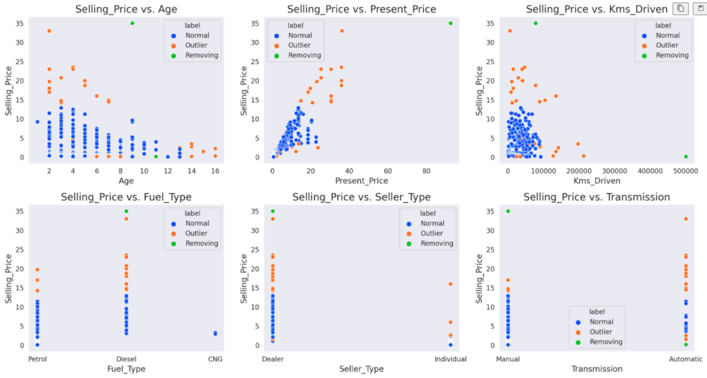
Let’s see the perfect outliers
removing_indexes = list(set(removing_indexes))
removing_indexes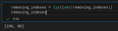
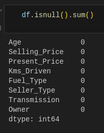
We got 2. We have to remove them. But before that we have to check if there’s any null data in our dataset.
df.isnull().sum()There are no null values in our dataset.
Let’s remove the identified outliers and reset the index of the dataframe.
df1 = df.copy()
df1.drop(removing_indexes, inplace=True)
df1.reset_index(drop=True, inplace=True)
Analysis of Dataset
Let’s analyze the data to see how much each field/category is correlated with the selling price of the car. We need to do some analysis on our dataset, to define some conclusion out of it.
To do that, we have to identify the numerical and categorical fields in our dataset. Because, the way to plot this differs for each type.
NumCols = ['Age', 'Selling_Price', 'Present_Price', 'Kms_Driven', 'Owner']
CatCols = ['Fuel_Type', 'Seller_Type', 'Transmission']
Selling Price vs Numerical Features Bivariate Analysis
fig, ax = plt.subplots(nrows=2 ,ncols=2, figsize=(10,10), dpi=90)
num_features = ['Present_Price', 'Kms_Driven', 'Age', 'Owner']
target = 'Selling_Price'
c = '#0055ff'

for i in range(len(num_features)):
    row = i//2
    col = i%2
    ax[row,col].scatter(df1[num_features[i]], df1[target], color=c, edgecolors='w', linewidths=0.25)
    ax[row,col].set_title('{} vs. {}'.format(target, num_features[i]), size = 12)
    ax[row,col].set_xlabel(num_features[i], size = 12)
    ax[row,col].set_ylabel(target, size = 12)
    ax[row,col].grid()

plt.suptitle('Selling Price vs. Numerical Features', size = 20)
plt.tight_layout()
plt.show()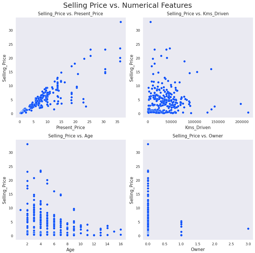
Selling Price vs Categorical Features Bivariate Analysis
fig, axes = plt.subplots(nrows=1 ,ncols=3, figsize=(12,5), dpi=100)
cat_features = ['Fuel_Type', 'Seller_Type', 'Transmission']
target = 'Selling_Price'
c = '#0055ff'

for i in range(len(cat_features)):
    sns.stripplot(ax=axes[i], x=cat_features[i], y=target, data=df1, size=6, color=c)
    axes[i].set_title('{} vs. {}'.format(target, cat_features[i]), size = 13)
    axes[i].set_xlabel(cat_features[i], size = 12)
    axes[i].set_ylabel(target, size = 12)
    axes[i].grid()

plt.suptitle('Selling Price vs. Categorical Features', size = 20)
plt.tight_layout()
plt.show()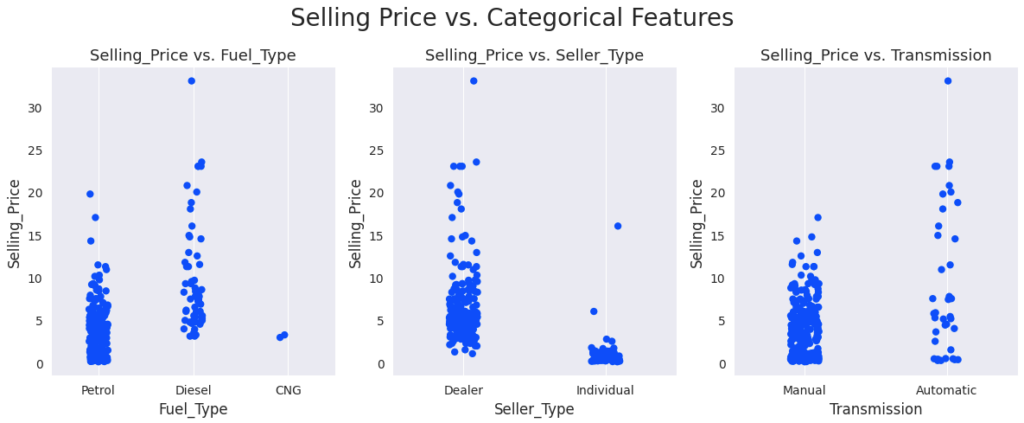
Here are the conclusion we can make from our data analysis,
- As Present Price increases, Selling Price increases as well. They’re directly proportional
- Selling Price is inversely proportional to Kilometers Driven
- Selling Price is inversely proportional to the car’s age
- As the number of previous car owners increases, its Selling Price decreases. So Selling Price is inversely proportional to Owner
- Diesel Cars > CNG Cars > Petrol Cars in terms of Selling Price
- The Selling Price of cars sold by individuals is lower than the price of cars sold by dealers
- Automatic cars are more expensive than manual cars
Categorical Variables Encoding
The Categorical fields cannot be used as it is. It has to be converted to numbers. Because, machines can understand only numbers. To achieve that, we’ll do one-hot encoding for the categorical columns. Pandas offer get_dummies method to encode the columns.
CatCols = ['Fuel_Type', 'Seller_Type', 'Transmission']
df1 = pd.get_dummies(df1, columns=CatCols, drop_first=True)
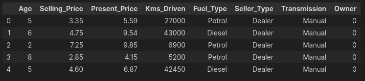
df1.head(5)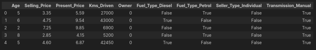
Assume True and False as 0 and 1 respectively.
Correlation Analysis
A correlation matrix is a matrix that summarizes the strength and direction of the linear relationships between pairs of variables in a dataset. It is a crucial tool in statistics and data analysis, used to examine the patterns of association between variables and understand how they may be related.
The correlation is directly proportional if the values are positive, and inversely proportional if the values are negative.
Here’s the code to find the correlation matrix with relation to Selling Price.
target = 'Selling_Price'
cmap = sns.diverging_palette(125, 28, s=100, l=65, sep=50, as_cmap=True)
fig, ax = plt.subplots(figsize=(9, 8), dpi=80)
ax = sns.heatmap(pd.concat([df1.drop(target,axis=1), df1[target]],axis=1).corr(), annot=True, cmap=cmap)
plt.show()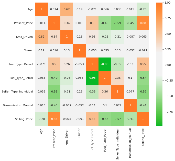
From the above matrix, we can infer that the target variable “Selling Price” is highly correlated with Present Price, Seller Type and Fuel Type.
Build Linear Regression Model
We have come to the final stage. Let’s train and test our model.
Let’s remove the “Selling_Price” from input and set it to output. This means that it has to be predicted.
X = df1.drop('Selling_Price', axis=1)
y = df1['Selling_Price']
Let’s split our dataset by taking 70% of data for training and 30% of data for testing.
X_train, X_test, y_train, y_test = train_test_split(X, y, test_size=0.3, random_state=0)Let’s take a backup of our test data. We need this for final comparison.
y_test_actual = y_testNormalize the dataset
The StandardScaler is a preprocessing technique commonly used in machine learning and data analysis to standardize or normalize the features (variables) of a dataset. Its primary purpose is to transform the data such that each feature has a mean (average) of 0 and a standard deviation of 1.
Let’s normalize our dataset using StandardScaler.
scaler = StandardScaler()
scaler.fit(X_train)
X_train_scaled = scaler.transform(X_train)
X_test_scaled = scaler.transform(X_test)
It is very important that StandardScaler transformation should only be learnt from the training set, otherwise it will lead to data leakage.
Train the model
linear_reg = LinearRegression()
linear_reg.fit(X_train_scaled, y_train)
Let’s find the intercept and co-efficient for each column in our training dataset.
pd.DataFrame(data = np.append(linear_reg.intercept_ , linear_reg.coef_), index = ['Intercept']+[col+" Coef." for col in X.columns], columns=['Value']).sort_values('Value', ascending=False)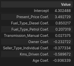
Evaluate the model
def model_evaluation(model, X_test, y_test, model_name):
    y_pred = model.predict(X_test)

    MAE = metrics.mean_absolute_error(y_test, y_pred)
    MSE = metrics.mean_squared_error(y_test, y_pred)
    RMSE = np.sqrt(MSE)
    R2_Score = metrics.r2_score(y_test, y_pred)

    return pd.DataFrame([MAE, MSE, RMSE, R2_Score], index=['MAE', 'MSE', 'RMSE' ,'R2-Score'], columns=[model_name])

model_evaluation(linear_reg, X_test_scaled, y_test, 'Linear Reg.')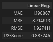
Model Evaluation using Cross-Validation
K-Fold Cross-Validation
In k-fold cross-validation, the dataset is divided into k roughly equal-sized subsets or “folds.” The model is trained and evaluated k times, each time using a different fold as the validation set and the remaining folds as the training set. The results (e.g., accuracy, error) of these k runs are then averaged to obtain a more robust estimate of the model’s performance. The advantage is that each data point is used for both training and validation, reducing the risk of bias in the evaluation.
linear_reg_cv = LinearRegression()
scaler = StandardScaler()
pipeline = make_pipeline(StandardScaler(),  LinearRegression())

kf = KFold(n_splits=6, shuffle=True, random_state=0)
scoring = ['neg_mean_absolute_error', 'neg_mean_squared_error', 'neg_root_mean_squared_error', 'r2']
result = cross_validate(pipeline, X, y, cv=kf, return_train_score=True, scoring=scoring)

MAE_mean = (-result['test_neg_mean_absolute_error']).mean()
MAE_std = (-result['test_neg_mean_absolute_error']).std()
MSE_mean = (-result['test_neg_mean_squared_error']).mean()
MSE_std = (-result['test_neg_mean_squared_error']).std()
RMSE_mean = (-result['test_neg_root_mean_squared_error']).mean()
RMSE_std = (-result['test_neg_root_mean_squared_error']).std()
R2_Score_mean = result['test_r2'].mean()
R2_Score_std = result['test_r2'].std()

pd.DataFrame({'Mean': [MAE_mean,MSE_mean,RMSE_mean,R2_Score_mean], 'Std': [MAE_std,MSE_std,RMSE_std,R2_Score_std]},
             index=['MAE', 'MSE', 'RMSE' ,'R2-Score'])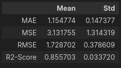
Results Visualization
Let’s create a dataframe with the actual and predicted values.
y_test_pred = linear_reg.predict(X_test_scaled)
df_comp = pd.DataFrame({'Actual':y_test_actual, 'Predicted':y_test_pred})
Let’s compare the actual and predicted target values for the test data with the help of a bar plot.
def compare_plot(df_comp):
    df_comp.reset_index(inplace=True)
    df_comp.plot(y=['Actual','Predicted'], kind='bar', figsize=(20,7), width=0.8)
    plt.title('Predicted vs. Actual Target Values for Test Data', fontsize=20)
    plt.ylabel('Selling_Price', fontsize=15)
    plt.show()

compare_plot(df_comp)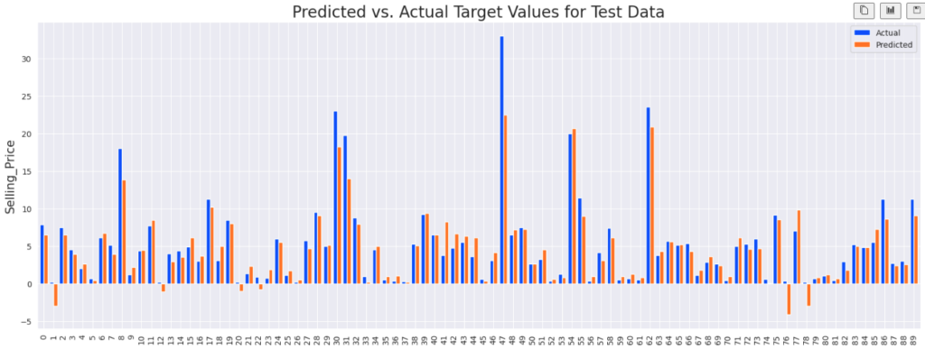
In the above graph, the blue lines indicates the actual price and orange lines indicate the predicted price of the cars. You can notice that some predicted values are negative. But in most of our cases, our model has predicted it pretty well.
This is not the perfect model. However if you want to fine tune it to make better predictions, please let me know via my email. I’ll write a blog about that if I receive more request.
Conclusion
In this blog, we have learnt about Linear Regression with a practical example. Hope it helps you to make progress in your ML journey. You can access the above dataset and the code for it in from this Github repo.
If you wish to learn more about artificial intelligence / machine learning / deep learning, subscribe to my article by entering your email address in the below box.
Have a look at my site which has a consolidated list of all my blogs.